Introduction to Error Analysis: The Science of Measurements, Uncertainties, and Data Analysis by Jack Merrin
Author:Jack Merrin
Language: eng
Format: mobi, epub
Published: 2017-08-30T07:00:00+00:00
4.2
The least squares method 4.2.1
Optimisation in calculus We can now see how curve fitting can be thought of as an optimization problem where you minimize some error function. Let’s review some concepts from calculus that allow us to perform optimization now.
Suppose we have a function f (x) and want to find the minimum value of the function over some range [a, b]. We know that local minima are critical points where f 0(x0) = 0 and the curva-ture is upwards f 00(x0) > 0.
Example 4.1. Find the critical points of f (x) = A + Bx +
Cx2. What condition is required for a global minimum.
Solution 4.1. We take the derivative f 0(x) = B + 2Cx0 = 0
x0 = −B/2C
For x0 to be a minimum, we require f 00(x0) = 2C > 0 or C > 0
4.2.2
Linear models The most basic model you can do a curve fit on is a straight line.
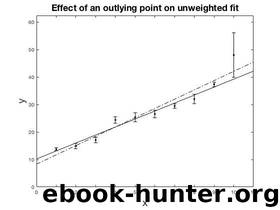
We will consider three models. The first is y = A + Bx this is the most general straight line. The second is a straight line through the origin y = Bx. The third is a horizontal line y = A.
This is also the same as averaging together the measurements and is known as the weighted mean. It is weighted because the experiments typically have different uncertainties and you put more preference towards the measurements with smaller uncertainties.
4.2. THE LEAST SQUARES METHOD
65
Linear model are more general. Basically any function behind the A and B or C is possible as long as they don’t depend on the fit parameters. The parabola y = A + Bx + Cx2 is a linear model also, which sounds kind of weird. You will get the hang of it once we start solving some models and learn what you can do analytically and what you cannot. Sometimes a model is nonlinear, but you can transform it to a linear one. The good news is that if everyone uses the least squares convention everyone will get the same results for the fit parameters and uncertainties for linear models. It is definitely a worthwhile endeavor and something every scientist should learn. You want to know what is under the hood of your statistics program that is doing all these calculations automatically. You should be able to at least check the software to see if you get the same results in some simple situations.
4.2.3
Optimisation of χ2
The error function E we considered before can use one more tweak. We want to weight the points that we know with smaller uncertainties to count more in the optimization and the points with large error bars to count less. To do this, instead of E we define χ2.
N
(y − f (x X
i, a))2
χ2 =
i
σ2
i=1
i
The weighting is 1
wi = σ2i This makes χ2 dimensionless. We use the notation that a give the smallest χ2. χ2 is always the starting point for curve fitting with the least squares convention.
66
CHAPTER 4. LINEAR LEAST SQUARES
Download
Introduction to Error Analysis: The Science of Measurements, Uncertainties, and Data Analysis by Jack Merrin.epub
This site does not store any files on its server. We only index and link to content provided by other sites. Please contact the content providers to delete copyright contents if any and email us, we'll remove relevant links or contents immediately.
| Biomathematics | Differential Equations |
| Game Theory | Graph Theory |
| Linear Programming | Probability & Statistics |
| Statistics | Stochastic Modeling |
| Vector Analysis |
Modelling of Convective Heat and Mass Transfer in Rotating Flows by Igor V. Shevchuk(6509)
Weapons of Math Destruction by Cathy O'Neil(6404)
Factfulness: Ten Reasons We're Wrong About the World – and Why Things Are Better Than You Think by Hans Rosling(4812)
A Mind For Numbers: How to Excel at Math and Science (Even If You Flunked Algebra) by Barbara Oakley(3358)
Descartes' Error by Antonio Damasio(3351)
Factfulness_Ten Reasons We're Wrong About the World_and Why Things Are Better Than You Think by Hans Rosling(3283)
TCP IP by Todd Lammle(3247)
Fooled by Randomness: The Hidden Role of Chance in Life and in the Markets by Nassim Nicholas Taleb(3191)
The Tyranny of Metrics by Jerry Z. Muller(3148)
Applied Predictive Modeling by Max Kuhn & Kjell Johnson(3130)
The Book of Numbers by Peter Bentley(3024)
The Great Unknown by Marcus du Sautoy(2747)
Once Upon an Algorithm by Martin Erwig(2703)
Easy Algebra Step-by-Step by Sandra Luna McCune(2686)
Lady Luck by Kristen Ashley(2627)
Police Exams Prep 2018-2019 by Kaplan Test Prep(2618)
Practical Guide To Principal Component Methods in R (Multivariate Analysis Book 2) by Alboukadel Kassambara(2590)
Linear Time-Invariant Systems, Behaviors and Modules by Ulrich Oberst & Martin Scheicher & Ingrid Scheicher(2462)
All Things Reconsidered by Bill Thompson III(2449)
