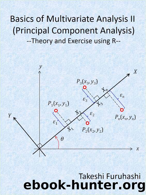
Basics of Multivariate Analysis II (Principal Component Analysis): Theory and Exercise using R by Takeshi Furuhashi

Author:Takeshi Furuhashi [Takeshi Furuhashi]
Language: eng
Format: epub
Published: 2015-08-04T16:00:00+00:00

The fourth script

x_centered <- scale (x_somatometry, apply(x_somatometry, 2, mean), c(1, 1)),

will center the data in each column in Table 2.2 (see Sec. 2.3 ). The term mean refers to an average, apply (a, 2, mean) is the R function to calculate the mean value of each column in matrix a, while 2 indicates a column (if this is 1, then a row is indicated instead). The output of the apply() function in this case is a two-dimensional (2D) vector. c(p, q) is also a 2Dl vector. IF p = q = 1, then each element of the vector is 1. The function scale(x, mean, v) extracts the mean from x, and divides x by v. In the case of Table 2.2, x is a 20 × 2 matrix, and the mean and v are 2 × 1 vectors. From each element in the first column of x, the value in the first row of the mean is subtracted, and the resulting value is divided by the value in the first row of v. Because the value in the first row of c(1, 1) is 1, this does not change the value of the dividend.

By executing the plot() function below

plot(x_centered[,1],x_centered[,2],col=“red”, pch=1),

the distribution in Fig.2.10 (see Subsec.2.3.1 ) is obtained. After this data centering is complete, the scripts for the PC analysis are the same as those in Sec.2.2 . Fig. 2.13 shows the identified PC axis.

Download

Copyright Disclaimer:
This site does not store any files on its server. We only index and link to content provided by other sites. Please contact the content providers to delete copyright contents if any and email us, we'll remove relevant links or contents immediately.